
R の gglot2 を使用して人口のグラフを作成してみました。
使用したデータは、長野市がクリエイティブ・コモンズ・ライセンス表示4.0国際(CC-BY4.0)ライセンスの下に公開している「長野市 令和5年地区別年齢別人口」(2023/01/13 更新)です。
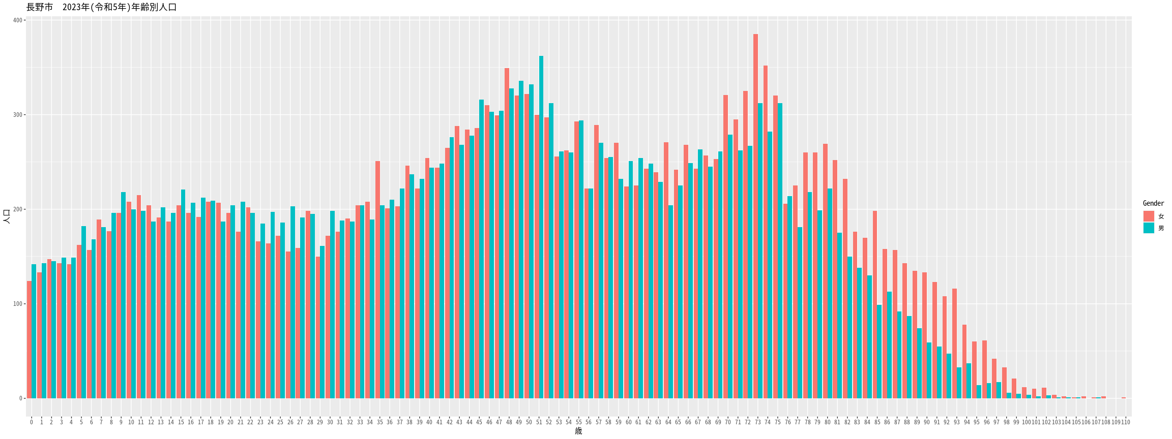
全体
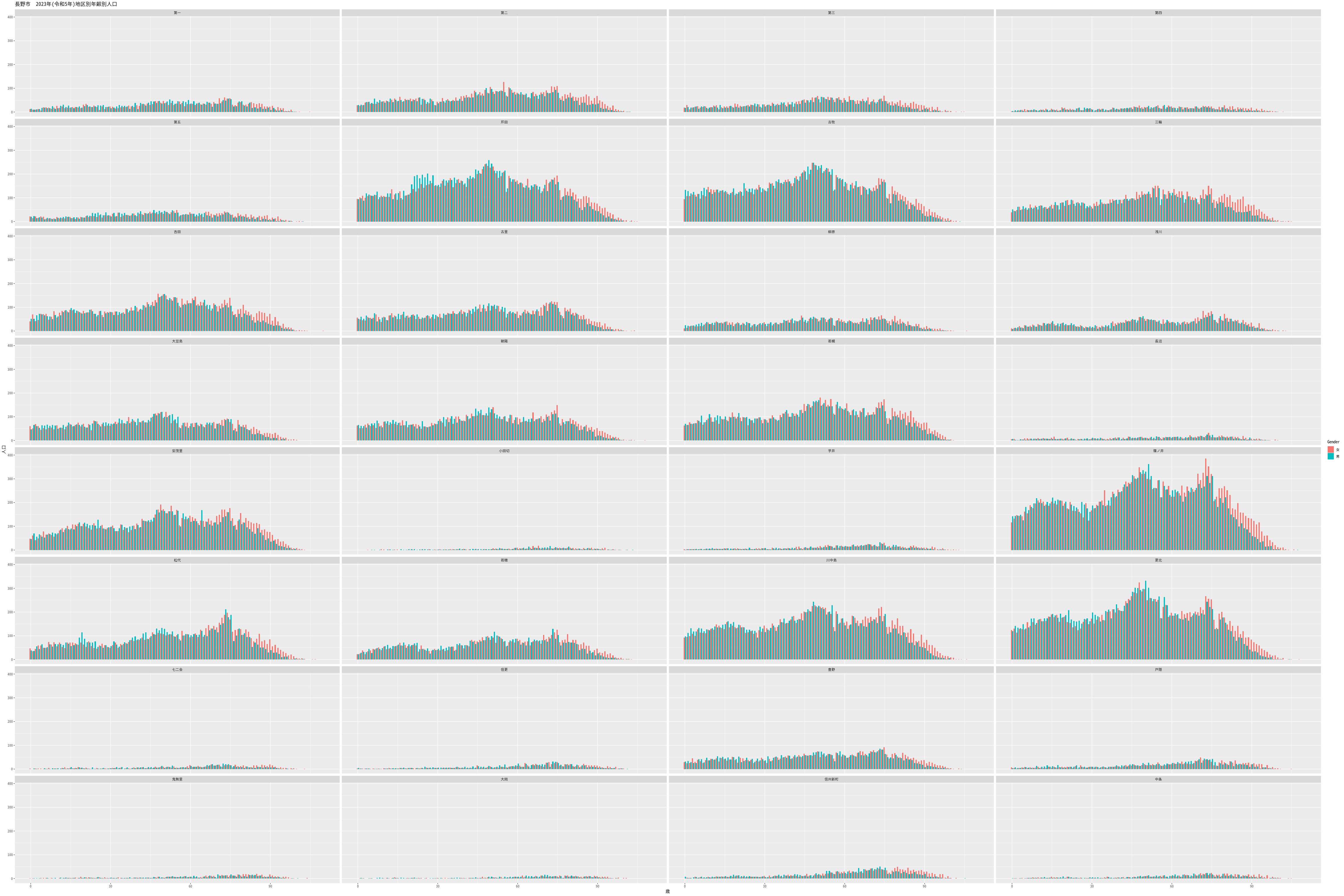
地区別
ソースコード
説明は、昨年の記事を参考にしてください。
library(tidyverse)

source("http://linkdata.org/api/1/rdf1s9823i/R")

data <- chikubetsu_nenreibetsu_202301[, -1]
area_levels = data[["地区名"]]
gender <- c("男","女")

cols <- data %>%
  colnames() %>%
  as.array()
ages <- cols[str_detect(cols, pattern="^X")] %>%
  str_extract(pattern="[0-9]+.+") %>%
  str_replace(pattern="(男|女)", "") %>%
  unique()

data2 <- data.frame()
for (r in 1:nrow(data)) {
  for (g in 1:length(gender)) {
    for (a in 1:length(ages)) {
      col <- sprintf("X%s%s", ages[a], gender[g])
      age <- as.numeric(str_replace(ages[a], "歳.*", ""))
      row <- c(
        data[r, "地区名"],
        gender[g],
        age,
        data[r, col]
      )
      data2 <- rbind(data2, row)
    }
  }
}
colnames(data2) <- c("Area", "Gender", "Age", "Population")
data2$Age <- as.numeric(data2$Age)
data2$Population <- as.numeric(data2$Population)
data2 <- data2 %>%
  mutate(Area = factor(Area, levels = area_levels))

theme_update(text=element_text(family="Noto Sans Mono CJK JP"))

options(repr.plot.width=24, repr.plot.height=9)
ggplot(data2, aes(x = as.factor(Age), y = Population, fill = Gender)) +
  geom_col(position = "dodge") +
  labs(title = "長野市 2023年(令和5年)年齢別人口", x = "歳", y = "人口")
ggsave("2023_nagano-shi_Population_All.png", width = 24, height = 9, dpi = 96)

options(repr.plot.width = 48, repr.plot.height = 32)
ggplot(data2, aes(x = Age, y = Population, fill = Gender)) +
  geom_col(position = "dodge") +
  facet_wrap(~Area, ncol = 4) +
  labs(title = "長野市 2023年(令和5年)地区別年齢別人口", x = "歳", y = "人口")
ggsave("2023_nagano-shi_Population_Area.png", width = 48, height = 32, dpi = 96)

コメント