
デフォルトの色で良ければ、そのままの方が無難なんですが、カテゴリ値を色で表したい場合があったので、その際のメモです。
データに色の列を足して scale_color_identity を使う
例としてデータは iris を使い、iris$Species をカテゴリ値とします。
iris$Speciesは、以下の様な factor です。

それぞれのカテゴリ値を、以下の色でプロットするとします。
実際のデータでは NA があることを想定して、「その他」の色も決めています。
- setosa : 赤
- versicolor : 黄
- virginica : 青
- その他 : 緑
ということで、対応する factor を定義します。
factor にしているのは、凡例を決まった並びにしたい為です。
palette <- factor(
  c("red", "yellow", "blue", "green"),
  levels = c("red", "yellow", "blue", "green")
)
データに色の列を追加します。
iris$Species の “setosa” は NA に置換しました。
定義はされていても、データには存在しないカテゴリ値という想定です。
列 “iro” に、そのプロットの色を設定します。
iris_with_color <- iris %>%
  mutate(Species = as.character(Species)) %>%
  mutate(Species = if_else(Species == "setosa", as.character(NA), Species)) %>%
  mutate(Species = factor(Species, levels = c("setosa", "versicolor", "virginica"))) %>%
  mutate(iro = case_when(
    Species == "setosa" ~ palette[1],
    Species == "versicolor" ~ palette[2],
    Species == "virginica" ~ palette[3],
    T ~ palette[4]
  ))
プロットしてみます。
ggplot(
  iris_with_color,
  aes(
    x = Sepal.Length,
    y = Sepal.Width,
    colour = iro
  )) +
  geom_point() +
  scale_color_identity(
    name = "Species",
    labels = c(
      "red" = "setosa",
      "yellow" = "versicolor",
      "blue" = "virginica",
      "green" = "unknown"
    ),
    guide = "legend"
  )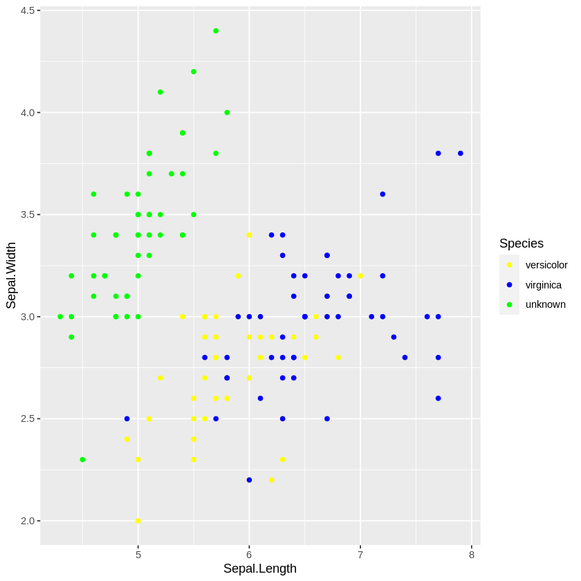
データが無いので、凡例に “setosa” がありません。
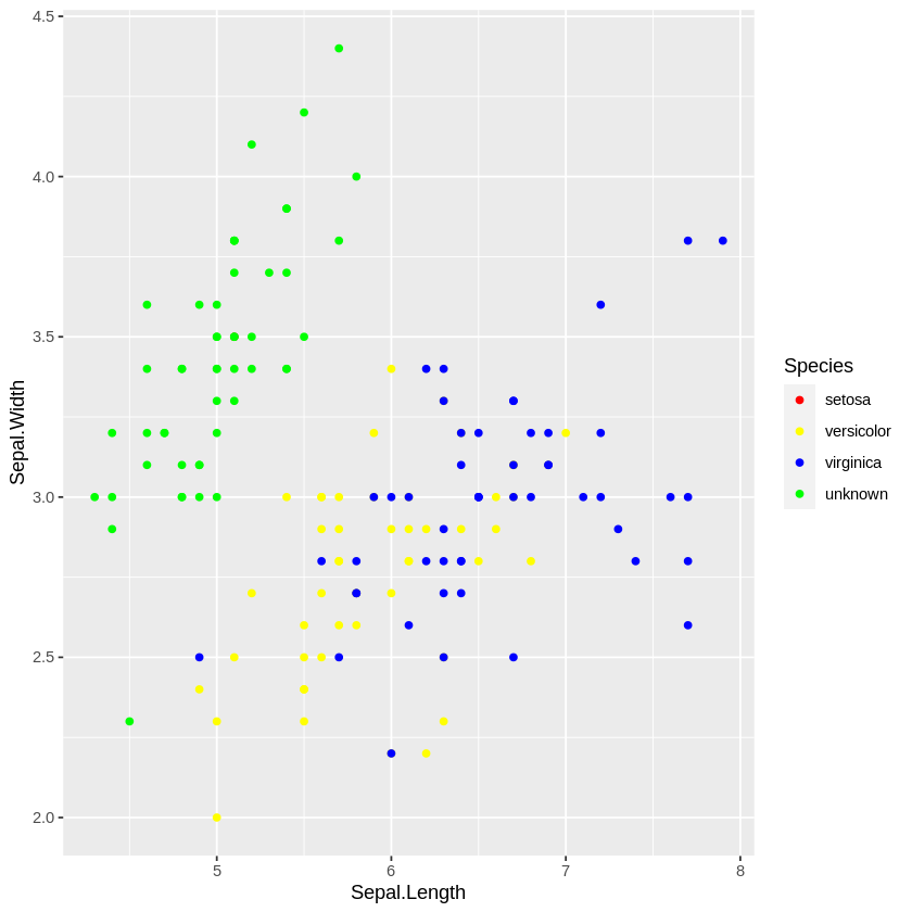
データが無くても、凡例には表記が欲しかったので、他のプロットに上書きされるデータとして混ぜることで実現してみました。
本来なら Species の種類分のダミーのデータを作るべきですが、以下では “setosa” だけ足しています。
もっと他に良い方法はあるんでしょうか。。
ggplot(
  iris_with_color[1,] %>%
    mutate(
      Species = "setosa",
      iro = palette[1]
    ) %>%
    rbind(iris_with_color),
  aes(
    x = Sepal.Length,
    y = Sepal.Width,
    colour = iro
  )) +
  geom_point() +
  scale_color_identity(
    name = "Species",
    labels = c(
      "red" = "setosa",
      "yellow" = "versicolor",
      "blue" = "virginica",
      "green" = "unknown"
    ),
    guide = "legend"
  )
最終的なコードは以下の通りです。
library(ggplot2)
library(dplyr)

palette <- factor(
  c("red", "yellow", "blue", "green"),
  levels = c("red", "yellow", "blue", "green")
)

iris_with_color <- iris %>%
  mutate(Species = as.character(Species)) %>%
  mutate(Species = if_else(Species == "setosa", as.character(NA), Species)) %>%
  mutate(Species = factor(Species, levels = c("setosa", "versicolor", "virginica"))) %>%
  mutate(iro = case_when(
    Species == "setosa" ~ palette[1],
    Species == "versicolor" ~ palette[2],
    Species == "virginica" ~ palette[3],
    T ~ palette[4]
  ))

ggplot(
  iris_with_color[1,] %>%
    mutate(
      Species = "setosa",
      iro = palette[1]
    ) %>%
    rbind(iris_with_color),
  aes(
    x = Sepal.Length,
    y = Sepal.Width,
    colour = iro
  )) +
  geom_point() +
  scale_color_identity(
    name = "Species",
    labels = c(
      "red" = "setosa",
      "yellow" = "versicolor",
      "blue" = "virginica",
      "green" = "unknown"
    ),
    guide = "legend"
  )

コメント