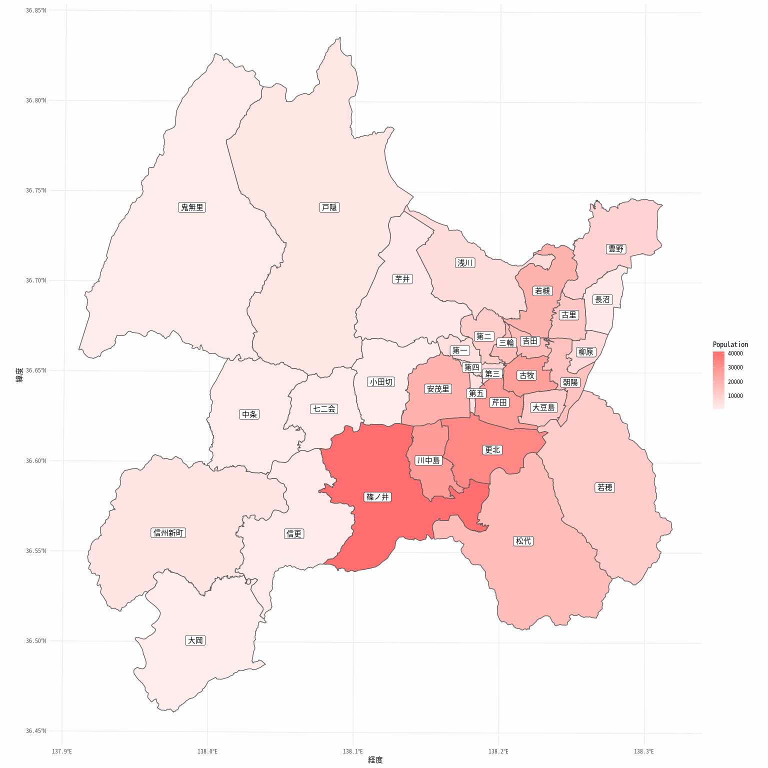
2022年5月長野市地区別人口
使用したデータは以下になります。
- 長野市 行政地図情報 で公開されていた「統計マップ」(令和3年4月1日)
- 「長野市 令和4年地区別年齢別人口」(2022/05/20 更新)
ソースコード
実行した環境は Google Colab です。
Google Drive からファイル取得が可能と知ったので、統計マップの 365179.zip は予め格納しています。
library(tidyverse)

# https://github.com/r-spatial/sf/issues/1572#issuecomment-758858154
system('sudo add-apt-repository ppa:ubuntugis/ubuntugis-unstable')
system('sudo apt-get update')
system('sudo apt-get install libudunits2-dev libgdal-dev libgeos-dev libproj-dev')
install.packages('sf')
library(sf)
必要なパッケージの読み込みです。
sf パッケージを使う為に、issue を参考に apt-get でパッケージをインストールしています。
system("apt-get install -y fonts-noto-cjk")
systemfonts::system_fonts()
theme_update(text=element_text(family="Noto Sans Mono CJK JP"))
日本語フォントを取得します。グラフの文字化けを回避する為です。
install.packages("R.utils")
library(R.utils)
library(httr)
library(googledrive)
reassignInPackage("is_interactive", pkgName = "httr", function() { return(TRUE) })
options(rlang_interactive=TRUE)
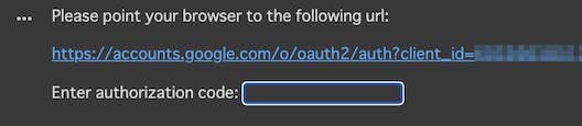
drive_auth(use_oob = TRUE, cache = FALSE)
Google Drive を使う為に認証します。
以下のように指示されるので、URL を開いて認証コードを取得し、そのコードを入力します。
drive_ls("Colab Notebooks") %>% select(name)
Google Drive が使えるか、試しに「Colab Notebooks」フォルダのファイル一覧を取得してみます。
# https://www.city.nagano.nagano.jp/soshiki/jouhou/114514.html
drive_get("Colab Notebooks/365179.zip") %>% drive_download(overwrite = TRUE)
Google Drive に保存した統計マップの zip ファイルを Google Colab にダウンロードします。
system("unzip -O sjis 365179.zip")
nagano_city <- read_sf("/content/支所所管区域(参考図)/R03支所所管区域.shp")
zip ファイルを解凍し、シェイプファイルを読み込みます。
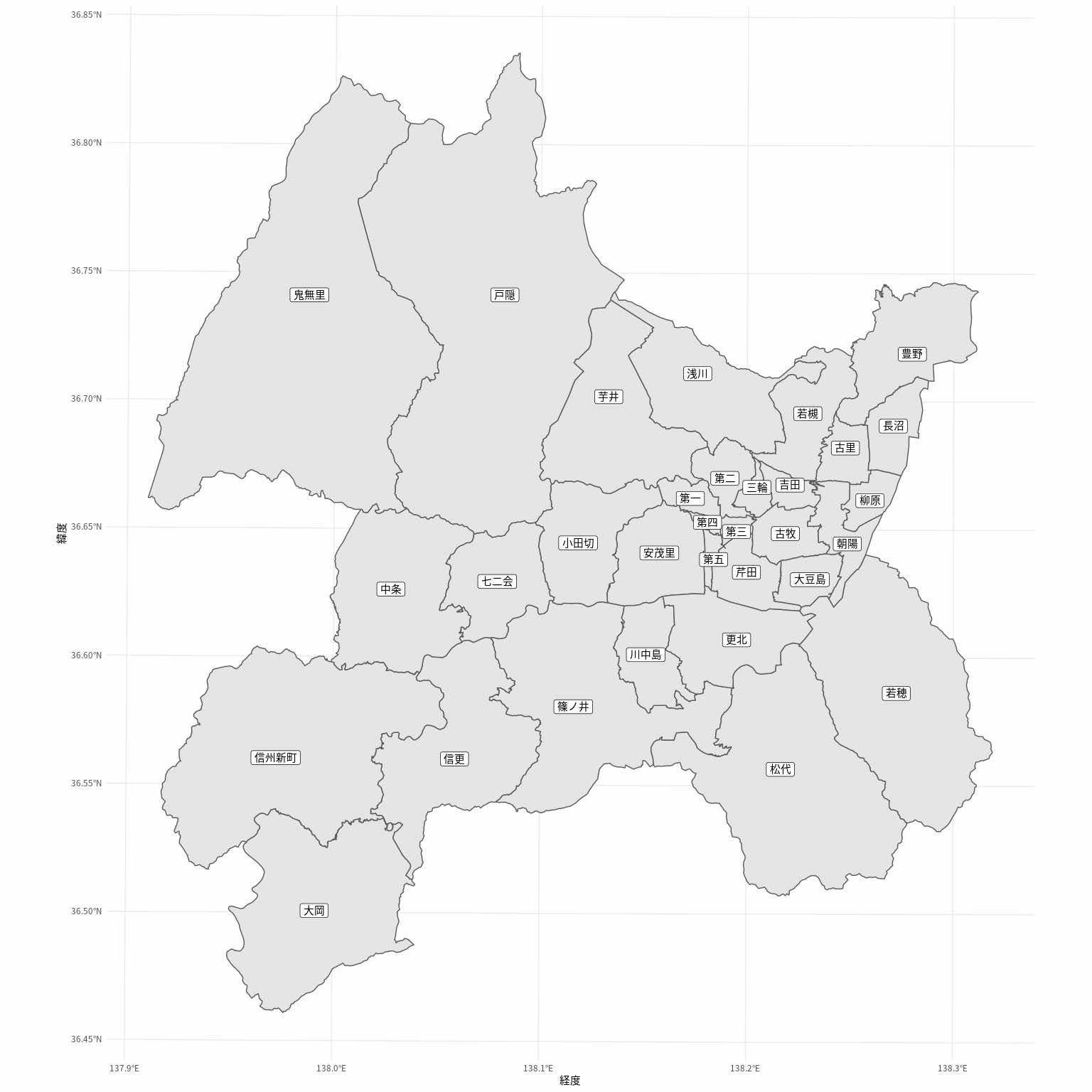
取得したデータで以下のように描画できます。
options(repr.plot.width = 16, repr.plot.height = 16)
ggplot(nagano_city) +
  geom_sf() +
  geom_sf_label(aes(label = 地区名)) +
  labs(x = "経度", y = "緯度") +
  theme_minimal() +
  theme(text=element_text(family="Noto Sans CJK JP"))
人口のデータも含まれていたのですが、昨年の数なので更新します。
data3 <- data2 %>%
  dplyr::group_by(Area) %>%
  dplyr::summarise(Population=sum(Population)) %>%
  dplyr::select(Area, Population)
data3$Area <- as.character(data3$Area)
data2 は「長野市 令和4年地区別年齢別人口」が入っています。
取得方法は前回と同様です。
data3 に地区別の人口を集計します。
nagano_city202205 <- data3 %>%
  dplyr::inner_join(nagano_city, by = c("Area" = "地区名")) %>%
  dplyr::select(Area, Population, geometry) %>%
  st_as_sf()
人口とマップのデータを結合します。
options(repr.plot.width = 16, repr.plot.height = 16)
ggplot(nagano_city202205) +
  geom_sf(aes(fill = Population)) +
  geom_sf_label(aes(label = Area)) +
  scale_fill_gradient(low = "#ffeeee", high = "#ff6e6e") +
  labs(x = "経度", y = "緯度") +
  theme_minimal() +
  theme(text=element_text(family="Noto Sans Mono CJK JP"))
ggsave("2022_nagano-shi_Population_Map.png", width = 16, height = 16, dpi = 96)
本投稿にある最初のマップになります。
更に、昨年との差でマップにしてみます。
nagano_city2205_2104 <- data3 %>%
  dplyr::inner_join(nagano_city, by = c("Area" = "地区名")) %>%
  dplyr::mutate(diff = Population - 人口_計) %>%
  dplyr::select(Area, diff, geometry) %>%
  st_as_sf()

options(repr.plot.width = 16, repr.plot.height = 16)
ggplot(nagano_city2205_2104) +
  geom_sf(aes(fill = diff)) +
  geom_sf_label(aes(label = Area)) +
  scale_fill_gradient2(low = "#6e6eff", mid = "#ffffff", high = "#ff6e6e") +
  labs(x = "経度", y = "緯度") +
  theme_minimal() +
  theme(text=element_text(family="Noto Sans CJK JP"))
  ggsave("2022_nagano-shi_Population_Map1.png", width = 16, height = 16, dpi = 96)
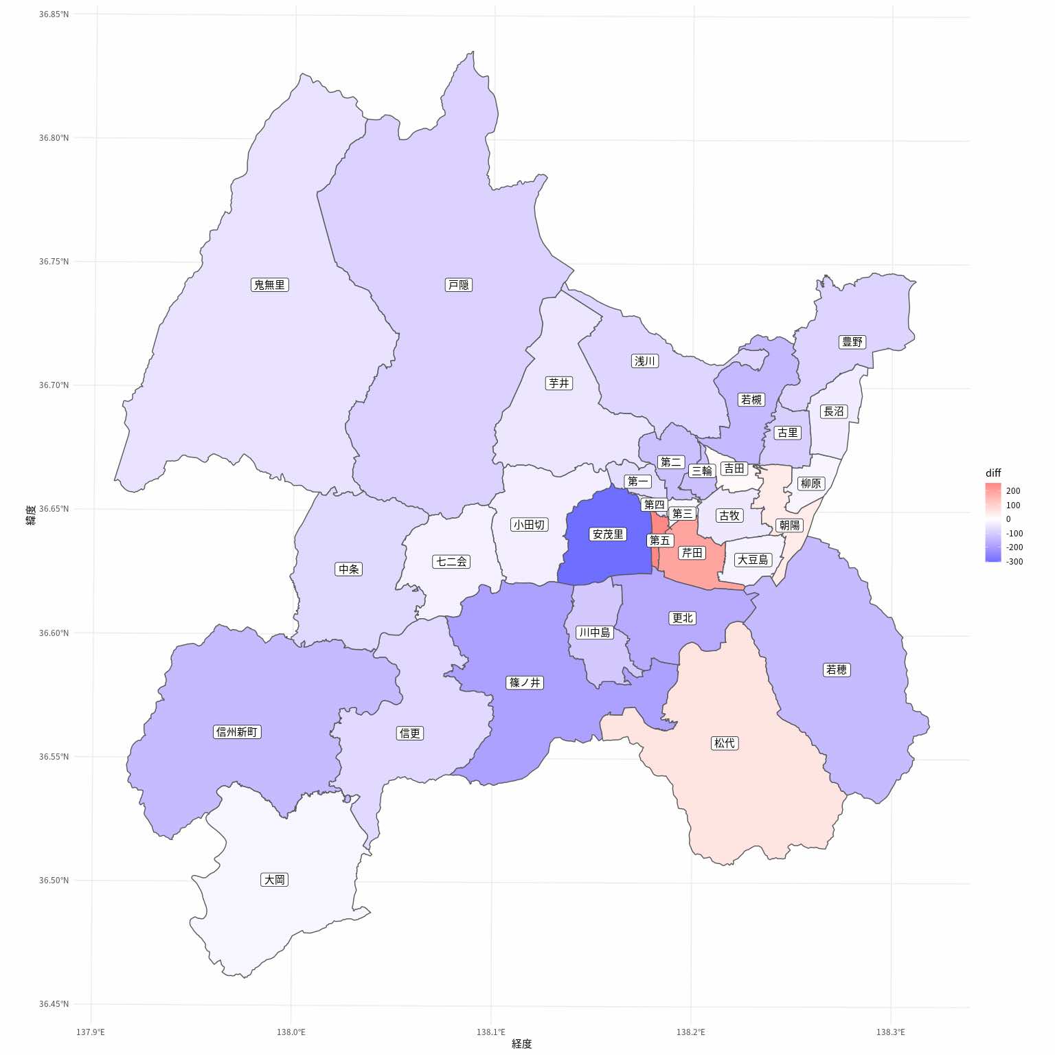
長野市地区別人口増減(2021年4月〜2022年5月)
データ分析のためのデータ可視化入門 (Amazon)